
Bob the lazy builder doesn’t bother sorting his nails, screws, nuts, bolts, washers etc. They’re all muddled together in the bottom of his toolbox. Whenever Bob takes on a new job, he rummages around in his toolbox to see if he has everything he needs.
Despite this lack of organization, Bob’s services are in demand. His business is growing and so is his toolbox, to the point that rummaging around in it is taking up too much of his time. This article discusses various algorithms Bob could use and compares their efficiency. We shall make use of the C++ Standard Library and consider what its complexity guarantees mean to us in practice.
Modeling the Problem
Let’s use the term “widget” for any of the objects in Bob’s toolbox. For Bob’s purposes two widgets are the same if they have the same physical characteristics—size, material, shape etc. For example, all 25mm panel pins are considered equal. In programming terms we describe a widget as a value-based object. We can model this value using an int, which gives us the following:
  class widget
  {
  public: // Construct
    explicit widget(int value);
  public: // Access
    int value() const;
  public: // Compare
    bool operator==(widget const & other) const;
  private:
    int value_;
  };
The implementation of this simple class holds no surprises.
We’ll model the toolbox and the job using a standard container. Let’s also introduce a typedef for iterating through this container.
  typedef std::vector<widget> widgets;
  typedef widgets::const_iterator widget_it;
What Bob needs to know before starting on a job is:
  // Can the job be done using this toolbox?
  // Returns True if there's a widget in the toolbox for every
  // widget in the job, false otherwise.
  bool
  can_he_fix_it(widgets const & job, widgets const & toolbox);
Some Test Cases
None of the algorithms under consideration are any use unless they work, so first we’re going to set up some test cases. Although Bob’s real toolbox is large—containing tens of thousands of widgets—we can check our algorithms get the right answers using something much smaller. Note too that we make sure to test corner cases, such as the toolbox or the job being empty. These corner cases may not happen often but it would be an embarrassment to get them wrong.
For brevity, only one of the tests is included in full here.
  ....

  void test_repeated_widgets()
  {
    widget const tt[] = {
        widget(1), widget(2), widget(3),
        widget(2), widget(3), widget(1),
        widget(3), widget(1), widget(2)
    };
    widget const j1[] = {
      widget(3), widget(2),
      widget(2), widget(1),
      widget(1), widget(3)
    };
    widget const j2[] = {
      widget(4), widget(2),
      widget(2), widget(1),
      widget(1), widget(4)
    };
    widgets toolbox(tt, tt + sizeof tt / sizeof tt[0]);
    widgets job1(j1, j1 + sizeof j1 / sizeof j1[0]);
    widgets job2(j2, j2 + sizeof j2 / sizeof j2[0]);
    assert(can_he_fix_it(job1, toolbox));
    assert(!can_he_fix_it(job2, toolbox));
  }

  void test_can_he_fix_it()
  {
    test_empty_toolbox();
    test_empty_job();
    test_job_bigger_than_toolbox();
    test_repeated_widgets();
    ....
  }
Complexity and the C++ Standard Library
In discussing the complexity of an algorithm, we’ll be using big O notation. We characterize an algorithm’s complexity in terms of the number of steps it takes, and how many more steps it takes as the size of the algorithm’s inputs increase.
So, for example, obtaining the value of an entry in an array of size N takes the same amount of time, no matter how big N is. We just add the index to base address of the array and read the value directly. This behavior is described as constant time, or O(1). If, instead, we’re looking for a value in a linked list of size N we have to step through the links one by one. On average, we’ll need to follow N/2 links. This behavior is linear, or O(N)—notice that we often omit any constant factors when describing the complexity of an algorithm.
Algorithms such as binary search, which repeatedly split the input data in half before arriving at an answer, are of logarithmic complexity. Consider, for example, looking up a word in a dictionary. We open the book at the middle: if we’ve found the word, we’re done, otherwise, since the dictionary is ordered, we know the word must be in the first or second half of the dictionary; thus, having halved the number of pages to search through, we can repeat the process until we find the word. We see this behavior often in the associative containers from the Standard Library, which typically use balanced binary trees to store their values. The depth of the tree is proportional to the logarithm of the size of the container; hence the complexity of, for example, a std::map read operation, is logarithmic.
As input sizes grow larger the higher order terms in big O notation come to dominate. Thus, if an algorithm takes 1000 * log(N) + N steps, as N gets larger the logarithmic term is dwarfed by the linear term. The algorithm is, therefore, simply O(N).
The C++ Standard Library1 does not mandate how its various algorithms and containers should be implemented: rather, it lays down preconditions for their use, in return giving us guarantees about both their results and the number of steps taken to achieve these results. Sometimes these guarantees are precise: for example, the complexity of for_each(first, last, op) is linear, applying op exactly first - last times. Sometimes an operation’s behavior needs to be averaged out over a number of calls: for example, the complexity of push_back on a vector is amortized constant time, since every so often it may be necessary to reallocate storage, and, as a consequence, that particular call to push_back takes rather longer. And sometimes the behavior depends on the properties of the inputs: for example, constructing a unique sorted container from an input iterator range is, in general O(N * log(N)), but reduces to O(N) if the values in the iterator range are already sorted.
Let’s see how this works by coding some solutions to Bob’s toolbox problem and analyzing their complexity.
Brute Force
The first version of can_he_fix_it uses brute force. For each widget in the job we look in the toolbox to see if there’s a matching widget that we haven’t already used. If there isn’t, then we haven’t enough widgets to take on the job, and we know our answer must be false. If there is, mark the toolbox widget as used and continue on to the next widget in the job. If we reach the end of the job in this way without problems, we return true.
  // Strategy: For each widget in the job, iterate through the widgets
  // in the toolbox looking for a matching widget. If we find a match
  // which we haven't used already, make a note of it and continue to
  // the next job widget. If we don't, fail.
  bool
  can_he_fix_it(widgets const & job,
                widgets const & toolbox)
  {
    bool yes_he_can = true;
    // Track widgets from the toolbox which we've used already
    std::set<widget_it> used;
    widget_it const t_end = toolbox.end();

    for (widget_it j = job.begin(); yes_he_can && j != job.end(); ++j)
    {
      yes_he_can = false;
      widget_it t = toolbox.begin();
      while (!yes_he_can && t != t_end)
      {
        t = std::find(t, t_end, *j);
        yes_he_can = t != t_end && used.find(t) == used.end();
        if (yes_he_can)
        {
          used.insert(t++);
        }
        if (t != t_end)
        {
          ++t;
        }
      }
    }
    return yes_he_can;
  }
How does this algorithm perform? In the fastest case, the algorithm completes in just T steps. This would happen if the very first job widget isn’t in the toolbox. In this case, the call:
t = std::find(t, t_end, *j);
with t set to toolbox.begin() returns t_end, and then a couple of simple tests cause our function to exit the loop and return false. Now, the C++ Standard Library documentation tells us that the complexity of std::find is linear: we’ll be making at most t_end - t (and in this case exactly t_end - t) comparisons for equality. That’s because our toolbox is unsorted (indeed, we can’t sort it yet, because we haven’t defined a widget ordering). To find an element from a range, all std::find can do is advance through the range, one step at a time, testing each value in turn. By contrast, note that the find which appears on the next line of code:
used.find(t) == used.end();
is actually a member function of std::set. This particular find takes advantage of the fact that a set is a sorted container, and is of logarithmic complexity. Note here that although our widgets are unsorted—and, as yet, unsortable—random access iterators into the widgets vector can be both compared and sorted.
Generally, though, in complexity analysis, the fastest case isn’t of greatest interest: we’re more interested in the average case or even the worst case. In the worst case, then, we must work through all J widgets in the job, and for each of these widgets we have to find unique matches in the toolbox, requiring O(T) steps. For each successful comparison we also have to check in the set to see if we’ve already used this widget from the toolbox, which ends up being a O(log(J)) operation.
So, the complexity looks like:
O(J * T + J * log(J))
Assuming T is larger than J, as T and J grow larger the J * log(J) term becomes insignificant. Our algorithm is O(J * T). If, typically, a job’s size is 10% of the size of the toolbox, this algorithm takes O(T * T / 10) steps, and is, then, quadratic in T.
What does quadratic performance mean to Bob? Well, he doesn’t charge for a quotation, which is when he needs to consider if he has enough tools to take on a job. Quadratic performance has the unfortunate result that every time his toolbox doubles in size, generating this part of the quotation takes four times as long. Wasting time is costing Bob money. We shall have to do better than this!
Sort Then Compare
Our second strategy requires us to sort the job and the toolbox before we start comparing them. First, we’ll have to define an order on our widgets. We can do this by adding operator<() to the widget class:
bool operator<(widget const & other) const;
which we implement:
  bool widget::operator<(widget const & other) const
  {
    return value_ < other.value_;
  }
With this ordering in place, we can code the following:
  // Strategy: sort both the job and the toolbox.
  // Then iterate through the widgets in the sorted job.
  // For each widget value in the job, see how
  // many widgets there are of this value, then see if
  // we have enough widgets of this value in the toolbox.
  bool
  can_he_fix_it(widgets const & job,
                widgets const & toolbox)
  {
    widgets sorted_job(job);
    widgets sorted_toolbox(toolbox);
    std::sort(sorted_job.begin(), sorted_job.end());
    std::sort(sorted_toolbox.begin(), sorted_toolbox.end());

    bool yes_he_can = true;
    widget_it j = sorted_job.begin();
    widget_it const j_end = sorted_job.end();
    widget_it t = sorted_toolbox.begin();
    widget_it const t_end = sorted_toolbox.end();

    while (yes_he_can && j != j_end)
    {
      widget_it next_j = std::upper_bound(j, j_end, *j);
      std::pair<widget_it, widget_it> matching_tools
        = std::equal_range(t, t_end, *j);
      yes_he_can
        = next_j - j <= matching_tools.second - matching_tools.first;
      j = next_j;
      t = matching_tools.second;
    }
    return yes_he_can;
  }
Sorting is easy—the standard library algorithm std::sort handles it directly. Sorting has O(N log N) complexity, so this stage has cost us O(J log J) + O(T log T) steps.
Once we have a sorted vector of job and toolbox widgets, we can perform the comparison in a single pass through the data. Now the data is sorted, we have an alternative to std::find when we want to locate items of a particular value. We can use binary search techniques to home in on a desired element. This is how std::equal_range and std::upper_bound work.
The call to equal_range(t, t_end, *j) makes at most 2 * log(t_end - t) + 1 comparisons. Similarly, the call to upper_bound(j, j_end, *j) takes at most log(j_end - j) + 1 comparisons.
The number times each of these functions gets called depends on how many unique widget values there are in the job. If all J widgets share a single value, we’ll call each function just once; and at the other extreme, if no two widgets in the job are equal, we may end up calling each function J times.
In the worst case, the comparison costs us something like O(J log J) + O(J log T) steps. We may well have been better off with plain old find—it really depends on how the widgets in a job/toolbox are partitioned. In any case, the total complexity is:
O(J log J) + O(T log T) + O(J log J) + O(J log T)
Assuming that T is much bigger than J, the headline figure for this solution is O(T log T). This will represent a very substantial saving over our first solution as T increases.
Before moving to our next implementation, it’s worth pointing out that once the toolbox has been sorted it stays sorted—. Bob could make even greater savings using a simple variant of this implementation if he changed the interface to can_he_fix_it to allow him to consider several jobs at a time.
Set Inclusion
The implementations of our first two algorithms have both been a little fiddly. We needed our test program to give us any confidence that they were correct. Our third implementation takes advantage of the fact that what we’re really doing is seeing if the job is a subset of the toolbox. By converting the inputs into sets (into multisets, actually, since any widget can appear any number of times in a job or a toolbox), we can implement our comparison trivially, using a single call to includes. It’s a lot easier to see how this solution works.
  // Strategy: copy the job and the toolbox into a multiset,
  // then see if the toolbox includes the job.
  bool
  can_he_fix_it(widgets const & job,
                widgets const & toolbox)
  {
    std::multiset<widget> const jset(job.begin(), job.end());
    std::multiset<widget> const tset(toolbox.begin(), toolbox.end());
    return std::includes(tset.begin(), tset.end(),
                         jset.begin(), jset.end());
  }
Our call to includes will make at most 2 * (T + J) - 1 comparisions. Have we, then, a linear algorithm? Unfortunately not, since constructing a multiset of size T is an O(T log T) operation—essentially, the data must be arranged into a balanced tree. Once again, then, assuming that T is much larger than J, we have an O(T log T) algorithm.
Both the second and the third solutions require considerable secondary storage to operate. The second solution duplicated its inputs; the third was even more profligate, since, in addition to this, it needed to create all of the std::multiset infrastructure linking up nodes of the container. Complexity analysis isn’t overly concerned with storage requirements, but real programs cannot afford to take such a casual approach. Often, a trade-off gets made between memory and speed—as indeed happened when we dropped the brute force approach, which required relatively little secondary storage. It turns out, though, in this particular case, we shall find an algorithm which does well on both fronts.
Vector Inclusion
As mentioned, a std::multiset is a relatively complex container. The innocent looking constructor:
std::multiset<widget> const tset(toolbox.begin(), toolbox.end());
is not only (in general) an O(T log T) operation—it also requires a number of dynamic memory allocations to construct the linked container nodes. Now, since std::includes does not insist that its input iterators are from a set, but merely from sorted ranges, we could use a sorted std::vector instead.
  // Strategy: copy the job and the toolbox into vectors,
  // sort these vectors, then see if the sorted toolbox
  // includes the sorted job.
  bool
  can_he_fix_it(widgets const & job,
               widgets const & toolbox)
  {
    widgets sj(job);
    widgets st(toolbox);
    std::sort(sj.begin(), sj.end());
    std::sort(st.begin(), st.end());
    return std::includes(st.begin(), st.end(),
                         sj.begin(), sj.end());
  }
Here, constructing the widget vector, sj, is a linear operation which requires just a single dynamic memory allocation; and similarly for st. These vectors can then be sorted using O(J log J) and O(T log T) operations respectively. As before, the call to std::includes is linear, though this time it may be fractionally quicker than the set-based version since iterating though a vector involves incremental additions rather than following pointers.
So, in theory, the “vector inclusion” implementation is, like the “set inclusion” implementation, an O(T log T) operation. In practice, as we shall find out later when we measure the performance of our various implementations, it turns out to beat the “set inclusion” implementation by a constant factor of roughly 10. So, although we often omit these constant factors when analysing the complexity of an algorithm, we must be careful not to forget their effect. The rule of thumb—to use std::vector unless there’s good reason not to—applies here. It turns out, however, that we can make a far bigger improvement when we consider the range of values a widget can take.
Count Widget Values
Any widget is defined by an integral value. In fact, the number of distinct widget values is rather small. Bob’s toolbox contains tens of thousands of widgets, but there are only a few hundred distinct values. Let’s add this crucial piece of knowledge to our widget class:
  class widget
  {
    // All widget values are in the range 0 .. max_value - 1
    enum { max_value = 500 };
    ....
  };
This allows the following implementation:
  namespace
  {
   // Store the widget counts in an array indexed by widget value,
   // and return the total number of widgets.
  widgets::size_type
  count_widgets(widgets const & to_count, unsigned * widget_counts)
  {
    for (widget_it w = to_count.begin(); w != to_count.end(); ++w)
    {
      ++widget_counts[w->value()];
    }
    return to_count.size();
  }
  }

  // Strategy: preprocess the job counting how many widgets there
  // are of each value. Then iterate through the toolbox, reducing
  // counts every time we find a widget we need.
  bool
  can_he_fix_it(widgets const & job,
                widgets const & toolbox)
  {
    unsigned job_widget_counts[widget::max_value];
    std::fill(job_widget_counts,
              job_widget_counts + widget::max_value, 0);
    widgets::size_type
      count = count_widgets(job, job_widget_counts);

    for (widget_it t = toolbox.begin();
         count != 0 && t != toolbox.end(); ++t)
    {
      int const tv = t->value();
      if (job_widget_counts[tv] != 0)
      {
        // We can use this widget. Adjust counts accordingly.
        --job_widget_counts[tv];
        --count;
      }
    }
    return count == 0;
  }
Here, the only secondary storage we need is for an array which holds widget::max_value unsigned integers. We initialize this array to hold widget counts for the job—for example, job_widget_counts[42] holds the number of widgets of value 42 we need. We can now iterate just once through the toolbox using job_widget_counts to track which widgets we still require for the job. If the total count ever drops to zero, we exit the loop, knowing we can take the job on. The complexity here is O(J) to initialize the counts array and O(T) to perform the comparison, giving an overall complexity of O(J + T), which reduces to O(T) if, as before, we assume that T is much bigger than J.
This then is linear. We can still do better, but only if we’re prepared to work at a higher level and change the way we model jobs and toolboxes.
Keep Widgets Counted
To beat a linear algorithm we’ll need to persuade Bob to track the widgets in his toolbox more closely.
  class counted_widgets
  {
  public:
    // Construct an empty collection of widgets.
    counted_widgets();
  public:
    // Add a number of widgets to the collection.
    void add(widget to_add, unsigned how_many);

    // Count up widgets of the given type.
    unsigned count(widget to_count) const;

    // Try and remove a number of widgets of the given type.
    // Returns the number actually removed.
    unsigned remove(widget to_remove, unsigned how_many);

    // Does this counted collection of widgets include
    // another such collection?
    bool includes(counted_widgets const & other) const;
  private:
    unsigned widget_counts[widget::max_value];
  };
This isn’t such a bad model, since when Bob replenishes his toolbox, he typically empties in bags containing known numbers of widgets, and most job specifications include a pre-sorted bill of materials.
If we now model both job and toolbox using instances of the new counted_widgets class, what used to be called can_he_fix_it is now implemented as toolbox.includes(job). This counted_widgets::includes member function can be handled directly by std::equal which guarantees to make at most widget::max_value comparisons. Since widget::max_value remains fixed as T and J increase, we have finally reduced our solution to a constant time algorithm, which the C++ Standard Library renders as a single line of code.
  bool
  counted_widgets::includes(counted_widgets const & other)
  {
    return std::equal(widget_counts,
                      widget_counts + widget::max_value,
                      other.widget_counts,
                      std::greater_equal<unsigned>());
  }
Matching Permutations
We can’t do better than constant time, but just for fun let’s see how much worse we could do if we picked the wrong standard library algorithms. Here’s a version of factorial complexity:
  bool
  can_he_fix_it(widgets const & job,
                widgets const & toolbox)
  {
    // Handle edge case separately: if the job's bigger than
    // the toolbox, we can't call std::equal later in this function.
    if (job.size() > toolbox.size())
    {
      return false;
    }
    widgets permed(toolbox);
    std::sort(permed.begin(), permed.end());
    widget_it const jb = job.begin();
    widget_it const je = job.end();

    bool yes_he_can = false;
    bool more = true;
    while (!yes_he_can && more)
    {
      yes_he_can = std::equal(jb, je, permed.begin());
      more = std::next_permutation(permed.begin(), permed.end());
    }
    return yes_he_can;
  }
This solution, like our set-based one, has the advantage of clarity. We simply shuffle through all possible permutations of the toolbox, until we find one whose first entries exactly match those in the job. If we weren’t already suspicious of this approach, running our tests exposes the full horror of factorial complexity. They now takes seconds, not milliseconds, to run, despite no test toolbox containing more than ten widgets.
Let’s suppose we have a toolbox containing 20 distinct widgets, and a job which consists of a single widget not in the toolbox. There are 20! permutations of the toolbox and only after testing them all does this algorithm complete and return false. If each permutation takes one microsecond to generate and test, then can_he_fix_it takes roughly 77 millennia to complete.
Factorial complexity is worse than exponential: in other words, for any fixed value of M, N! grows more quickly than N to the power of M.
Measurements
The conventional wisdom on optimization is not to optimize unless absolutely necessary; and even then, not to change any code until you’ve run some calibrated test runs first. This article isn’t really about optimization, it’s about analyzing the complexity of algorithms which use the C++ Standard Library. That said, we really ought to measure the performance of our different implementations.
As always, the actual timing tests yield some surprises. Tables 1 and 2 collect the results of running six separate implementations of can_he_fix_it on varying toolbox sizes. For each toolbox size, T, the test used a fixed job size J = T / 10, and then created 10 random (toolbox, job) pairs and ran each of them through each implementation 50 times. The figures in the tables represent the time in seconds for 500 runs of each trial algorithm.
The columns in the table contain timing figures for each of six implementations:
- brute force: for each widget in the job, try and find a widget in the toolbox
- sort then compare: copy job and toolbox into vectors, sort, then iterate through matching them up
- set inclusion: copy job and toolbox into multisets, then use
std::includes - vector inclusion: copy job and toolbox into vectors, sort, then use
std::includes - count widget values: create an array of job widget counts, then iterate through the toolbox
- keep widgets counted: remodel the job and toolbox as a hand-rolled
counted_widgetscontainer.
T |
Brute Force | Sort then Compare | Set Inclusion | Vector Inclusion | Count Widget Values | Keep Widgets Counted |
|---|---|---|---|---|---|---|
| 5000 | 24.123 | 3.113 | 29.513 | 3.032 | 0.063 | 0 |
| 10000 | 78.608 | 5.954 | 60.343 | 6.25 | 0.079 | 0 |
| 15000 | 170.578 | 9.079 | 95.812 | 9.31 | 0.126 | 0 |
| 20000 | 280.389 | 11.83 | 127.202 | 11.877 | 0.14 | 0 |
| 25000 | 371.829 | 13.576 | 143.672 | 13.796 | 0.172 | 0 |
| 30000 | 529.547 | 15.952 | 175.486 | 16.78 | 0.157 | 0 |
| 35000 | 718.25 | 18.736 | 209.843 | 19.937 | 0.221 | 0 |
| 40000 | 933.454 | 21.453 | 243.626 | 22.812 | 0.219 | 0 |
| 45000 | 1178.08 | 24.639 | 277.643 | 26.765 | 0.234 | 0 |
| 50000 | 1450.36 | 27.249 | 308.937 | 28.548 | 0.266 | 0 |
Table 1. GCC, O2 optimization, time 500 runs in seconds
Table 2 collects results for MSVC 2005 version 8.0.50727.42, on the same platform, Pentium P4 CPU, 3.00GHz, 1.00GB of RAM.
T |
Brute Force | Sort then Compare | Set Inclusion | Vector Inclusion | Count Widget Values | Keep Widgets Counted |
|---|---|---|---|---|---|---|
| 5000 | 19.999 | 2.484 | 21.641 | 2.656 | 0.063 | 0 |
| 10000 | 69.451 | 4.8 | 50.028 | 4.971 | 0.078 | 0 |
| 15000 | 150.422 | 7.048 | 84.856 | 7.518 | 0.108 | 0 |
| 20000 | 263.109 | 9.657 | 122.389 | 9.922 | 0.122 | 0 |
| 25000 | 409.278 | 11.906 | 159.094 | 12.484 | 0.141 | 0 |
| 30000 | 582.276 | 14.143 | 197.576 | 15.249 | 0.203 | 0 |
| 35000 | 779.512 | 16.64 | 232.935 | 17.625 | 0.235 | 0 |
| 40000 | 941.868 | 17.953 | 258.609 | 19.282 | 0.248 | 0 |
| 45000 | 1164.18 | 19.686 | 297.653 | 20.78 | 0.253 | 0 |
| 50000 | 1461.15 | 22.344 | 330.545 | 23.516 | 0.282 | 0 |
Table 2. MSVC 2005, /O2 optimization, time 500 runs in seconds
The most obvious surprise is the final column. The clock resolution on my platform (I used std::clock() to obtain times with a 1 millisecond resolution) simply wasn’t fine enough to notice any time taken by the “keep widgets counted” implementation. The algorithms perform so very differently it’s quite tricky to write a program comparing them head to head. In the end, I simply ran a one-off version of my timing program which just collected times for the fifth implementation. The results, shown in Table 3, indicate the algorithm is indeed constant time, with each call taking just half a microsecond.
T |
Keep Widgets Counted |
|---|---|
| 5000 | 0.516 |
| 10000 | 0.562 |
| 15000 | 0.562 |
| 20000 | 0.579 |
| 25000 | 0.561 |
| 30000 | 0.486 |
| 35000 | 0.532 |
| 40000 | 0.532 |
| 45000 | 0.545 |
| 50000 | 0.546 |
Table 3. GCC, -O2 optimization, time 1000000 runs in seconds
There appears to be little difference between MSVC and GCC performance: perhaps MSVC does a little better on the sorted vector based implementations—or perhaps the random widget generator gave significantly different inputs. I did not experiment with other more sophisticated compiler settings.
The std::multiset approach (implementation 2), while perhaps the simplest, was consistently worse, by a factor of about 10, than either of the sorted vector approaches—and in fact performed worse than the first brute force algorithm for small toolboxes. I have not investigated why, but would guess this is the overhead of creating the associative container infrastructure.
There is no significant difference between the “sort then compare” implementation and the “vector inclusion” implementation. If, for some reason, we couldn’t use either the “count widget values” or the “keep widgets counted” implementation, then the “vector inclusion” implementation would be the best, being both simple and (relatively) lean.
Graphs
Figure 1 shows the familiar parabolic curve, indicating that our analysis is correct, and our very first “brute force” implementation is indeed O(N * N).
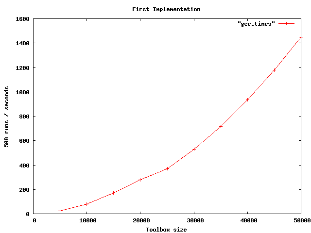
Figure 1. “Brute Force” Implementation
Figure 2 shows our second “sort then compare” implementation, which we analyzed to be O(N * log N). I haven’t done any detailed analysis or curve fitting, but see nothing to suggest our analysis is wrong.
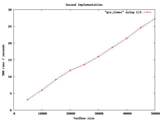
Figure 2. “Sort Then Compare” Implementation
Figure 3 shows our fourth “count widget values” implementation, which we analyzed to be O(N). Again, I haven’t done any detailed analysis or curve fitting. Clearly, the algorithm runs so fast that our test results are subject to timing jitter.
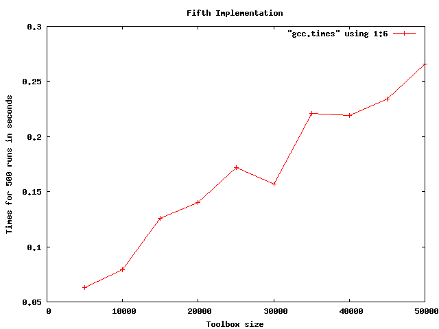
Figure 3. Times for “Count Widget Values” Implementation
Conclusions
This article has shown how we can use the C++ Standard Library to solve problems whilst retaining full control over efficiency. With a little thought we managed to reduce the complexity of our solution from N squared, through NlogN, to N, and finally to constant time. The real gains came from insights into the problem we were modeling, enabling us to choose the most appropriate containers and algorithms.
Much has been written about the perils of premature optimization, but Sutter and Alexandrescu remind us we shouldn’t pessimize prematurely either.2 Put simply: we wouldn’t be using C++ if we didn’t care about performance. The C++ Standard Library gives us the information we need to match the right containers with the right algorithms, keeping code both simple and efficient.
End Notes
1. The C++ Standard Library, ISO/IEC 14882.
2. Sutter, Alexandrescu, “C++ Coding Standards”, http://www.gotw.ca/publications/c++cs.htm
Resources
A zip file containing the code shown in this article can be downloaded here:
http://www.wordaligned.org/lazy_builder/index.html
The C++ Standard Library: A Tutorial and Reference, by Nicolai M. Josuttis, includes a discussion of algorithmic complexity. It is available from amazon.com at:
http://www.amazon.com/exec/obidos/ASIN/0201379260/
Bob the Builder's official website is here:
http://www.bobthebuilder.com
Credits
My thanks to the editorial team at The C++ Source for their help with this article.
The graphs were produced using GnuPlot (http://www.gnuplot.info/).
Talk back!
Have an opinion? Readers have already posted 9 comments about this article. Why not add yours?
About the author
Thomas Guest is an enthusiastic and experienced computer programmer. During the past 20 years he has played a part in all stages of the software development lifecycle—and indeed of the product development lifecycle. He's still not sure how to get it right. His website can be found at: http://homepage.ntlworld.com/thomas.guest
Artima provides consulting and training services to help you make the most of Scala, reactive
and functional programming, enterprise systems, big data, and testing.
2070 N Broadway Unit 305
Walnut Creek CA 94597
USA
(925) 918-1769 (Phone)